Covariance and Correlation

In many engineering and scientific applications, there are multiple variables involved. For instance, in structural engineering when assessing the health of a structure, we might have to take into account the different loads on the structure as well as the deterioration of the building materials. In climate science, when trying to study the effect of climate change in agricultural production, we might have to consider the impact of the changes in temperature, soil moisture and precipitation, amongst others, in vegetation.

These variables of interest are often “tied” to one another. For instance, the different variables to describe the wind loads on a building (e.g.: wind speed and wind direction) are generated by the same drivers and, thus, are dependent on each other. Also, the interest variables might be part of the same physical process: as temperature increases, some of the soil moisture evaporates, which might impact on the precipitation later.

In order to assess the streght of the dependence in these complex relationships between variables of interest, we can use statistical metrics for dependence. Here, we will discuss covariance and Pearson’s correlation coefficient.

Covariance: definition

Covariance is a measure of the joint variability of two variables. The definition of Covariance is given by

\[ \text{Cov}(X_1, X_2) = \mathbb{E}[(X_{1,i} - \mathbb{E}(X_1))(X_{2,i} - \mathbb{E}(X_2))] = \mathbb{E}(X_1 X_2)-\mathbb{E}(X_1)\mathbb{E}(X_2) \]

The covariance of two random variables can take both positive and negative values and has units equal to the product of the units of the analyzed variables. High absolute values of covariance imply a strong relationship between variables.

If \(Cov(X_1,X_2)>0\), high values of \(X_1\) typically occur together with high values of \(X_2\), while low values of \(X_1\) typically occur with low values of \(X_2\), therefore the covariance is defined as POSITIVE.

On the other hand, if \(Cov(X_1,X_2)<0\), high values of \(X_1\) typically occur together with low values of \(X_2\), while low values of \(X_1\) typically occur with high values of \(X_2\). In this case the covariance is defined as NEGATIVE.

Note that the covariance of one variable with itself is equal to the variance.

\[ Cov(X,X)=\mathbb{E}([X_i-\mathbb{E}(X)]^2) =Var(X)=\sigma^2_{X} \]

Covariance: geometric interpretation

In this section, we will see how to interpret the covariance as an average of geometric areas. Let’s see it with an example. Imagine that you are studying the relationship between the height and the Body Mass Index (\(BMI\)) of people. You have a short dataset with 20 observations that it is shown as a scatter plot in panel (a) of the image below.

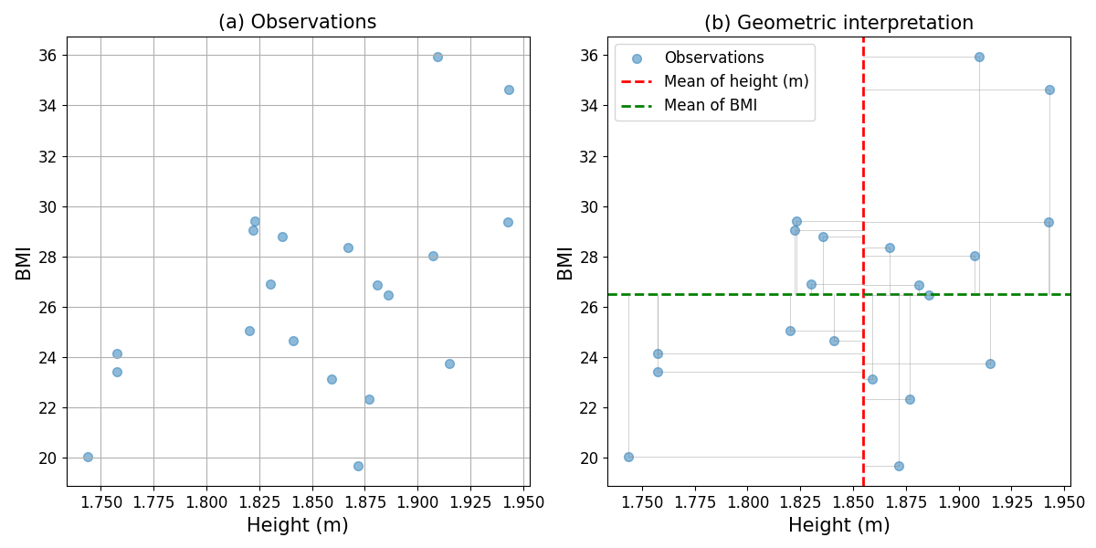
Fig. 1 Geometric interpretation of the covariance: (a) paired observations of height and BMI, and (b) rectangular areas defined by the observations and the mean values of the two random variables, which represent \([X_{1,i}-\mathbb{E}(X_1)][X_{2,i}-\mathbb{E}(X_2)]\).

We already introduced the definition of covariance as

\[ \text{Cov}(X_1, X_2) = \mathbb{E}[(X_{1,i} - \mathbb{E}(X_1))(X_{2,i} - \mathbb{E}(X_2))] \]

In that expression, we can see that the covariance is the expectation of a product of two terms. Each of these terms represents the difference or distance between an observation and the expected value of the random variable (i.e., its mean). Thus, each term can be graphically represented as a line that goes from the value of the observation to the mean. The product of the two defined distances can then be interpreted as the product of the sides of a rectangle which are defined by the distances of the observation to the mean values of the two random variables. This is, the areas of the rectangles defined in the panel (b) of the Figure above. The covariance is the expectation (or mean) of these areas, i.e. the covariance represents the average area of the defined rectangles, as shown in the figure below.

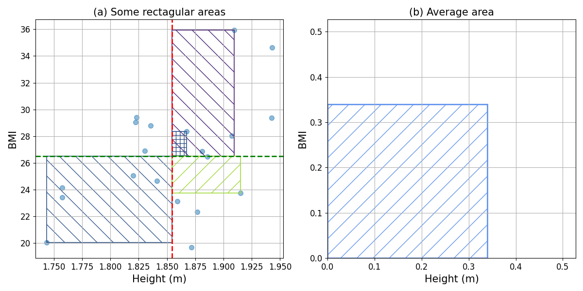
Fig. 2 Geometric interpretation of the covariance: (a) some of the areas that represent the term \([X_{1,i}-\mathbb{E}(X_1)][X_{2,i}-\mathbb{E}(X_2)]\), and (b) average area.

Covariance matrix

When considering a set of random variables, \(X_1, X_2, \ldots, X_m\), we can ‘collect’ all covariances in the so-called covariance matrix:

\[\begin{split} \Sigma_X= \left[\begin{array}{cccc} \sigma^2_1 & Cov(X_1,X_2) & \ldots & Cov(X_1,X_m) \\ Cov(X_1,X_2)& \sigma_{2}^2 & \ldots & Cov(X_2,X_m) \\\vdots & \vdots & \ddots & \vdots \\ Cov(X_1,X_m) & Cov(X_2,X_m) & \ldots & \sigma_{m}^2 \end{array}\right] \end{split}\]

Note that the covariance matrix is symmetric, since \(Cov(X_i,X_j)= Cov(X_j,X_i)\).

If all measurements are independent, all covariances will be equal to zero, and the covariance matrix becomes a diagonal matrix with the variances on the diagonal.

You will later use the covariance matrix when working with the multivariate Gaussian distribution.

Correlation

A drawback of the covariance is that it has units. In some situations, it is desirable to compare the stregth of the joint association between different pairs of random variables that do not necessarily have the same units. In those ocasions, correlation coefficients can be applied.

Pearson’s correlation coefficient is the most widely used correlation coefficient as it assesses the linear correlation between two random variables. Pearson’s correlation coeficient is defined as

\[ \rho = \frac{Cov(X_1, X_2)}{\sigma_{X_1}\sigma_{X_2}}=\frac{\sum_{i=1}^{n} (X_{1i} - \bar{X_1})(X_{2i} - \bar{X_2})}{\sqrt{\sum_{i=1}^{n} (X_{1i} - \bar{X_1})^2 \sum_{i=1}^{n} (X_{2i} - \bar{X_2})^2}} \]

where \(X_{1i}\) and \(X_{2i}\) are the individual data points for the random variables \(X_1\) and \(X_2\), respectively, \(\bar{X_1}\) and \(\bar{X_2}\) are the means of \(X_1\) and \(X_2\), and \(n\) is the number of data points.

The correlation coefficient takes values between -1 and 1, regardless the units of the random variables. If the random variables are uncorrelated or independent, \(\rho=0\). A positive correlation coefficient means that if one variable increases, the other one tends to increase. Conversely, a negative correlation means that an increase of one variable is accompanied by a tendency of the other variable to decrease. If the random variables are fully correlated (\(\rho=1\) or \(\rho=-1\)), it means that knowing the value of one variable implies that I know the value of the other variable being the relationship between them linear. In the figure below, you can see examples of how the samples for different correlation look.

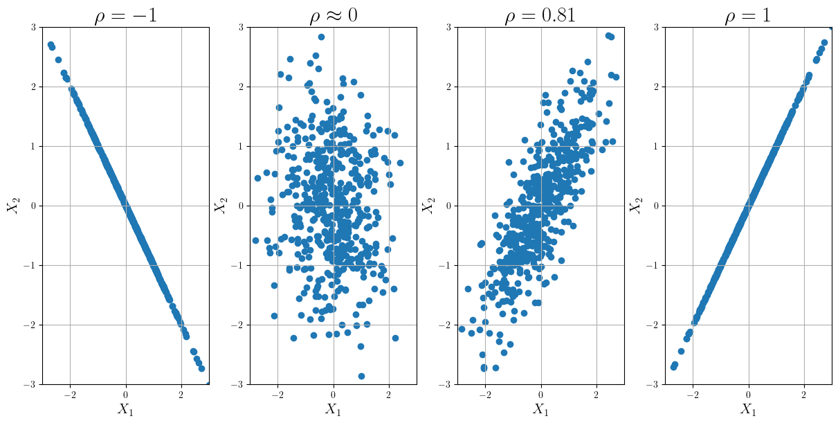
Fig. 3 Scatter plots for different values or Pearson’s correlation coefficient.

You can also play with the samples option in the interactive element below.