Multivariate Gaussian distribution

One of the simplest approaches to define a multivariate distribution, \(F(x_{1}, x_{2}..,x_{n})\), is through the multivariate Gaussian distribution. This model assumes that both the marginals and the dependence are Gaussian. Keep in mind that the Gaussian distribution might not always be the best model so its applicability is limited. However, it is a convenient model since it can be manipulated analytically and we can use it as a first approach to model the dependence. Here, emphasis is given in the simplest case of the multivariate Gaussian distribution, the bivariate distribution, as it is easier to visualize. However, the concepts explained here can be applied to Multivariate Gaussian distributions in higher dimensions.

Definition of bivariate Gaussian distribution

The bivariate Gaussian distribution for two random variables \(X_1\) and \(X_2\) is defined as

\[ \phi_{\rho}(x_1, x_2) = \frac{1}{2\pi \sigma_1 \sigma_2 \sqrt{1-\rho^2}} \exp \left( - \frac{\left( \frac{x_1-\mu_1}{\sigma_1}\right) -\left( \frac{2\rho (x_1-\mu_1)(x_2-\mu_2)}{\sigma_1 \sigma_2}\right) +\left(\frac{x_2-\mu_2}{\sigma_2} \right)}{2(1-\rho^2)}\right) \]

where \(x_1\) and \(x_2\) are values of the random variables, \(\sigma_1\) and \(\sigma_2\) are the standard deviations of the random variables, \(\rho\) is the correlation coefficient between \(X_1\) and \(X_2\), and \(\mu_1\) and \(\mu_2\) are the mean values of the random variables. Therefore, it has five parameters: \(\mu_1\), \(\mu_2\), \(\sigma_1\), \(\sigma_2\) and \(\rho\).

We can rewrite the above expression in matricial form as

\[\begin{split} \phi_{\rho}(x_1, x_2) = \frac{1}{\sqrt{(2\pi)^2 \begin{vmatrix} \sigma_1^2 \ \ \ \ Cov(X_1, X_2) \\ Cov(X_1, X_2) \ \ \sigma_2^2 \\ \end{vmatrix}}} \exp \left( -\frac{1}{2} (x_1 - \mu_1 \ x_2-\mu_2) \begin{pmatrix} \sigma_1^2 \ \ \ Cov(X_1, X_2) \\ Cov(X_1, X_2) \ \ \ \sigma_2^2 \end{pmatrix}^{-1} \begin{pmatrix} x_1 - \mu_1 \\ x_2 - \mu_2 \end{pmatrix} \right) \end{split}\]

where \(Cov(X_1, X_2)\) is the covariance of the random variables \(X_1\) and \(X_2\). We can also present the above form in a compressed fashion as

\[ \phi_{\rho}(x_1, x_2) = \frac{1}{\sqrt{(2\pi)^2 |\boldsymbol{\Sigma|}}} \exp{\left(-\frac{1}{2}(\boldsymbol{x-\mu})^T \boldsymbol{\Sigma}^{-1} (\boldsymbol{x-\mu})\right)} \]

where \(\boldsymbol{x}\) is the vector of values of the random variable, \(\boldsymbol{\mu}\) is the vector of means, and \(\boldsymbol{\Sigma}\) is the covariance matrix[1].

The cumulative distribution function of the bivariate Gaussian distribution would then be defined as

\[ \Phi_{X_1,X_2}(x_1,x_2)=P(X_1 \leq x_1, X_2 \leq x_2)=\int_{-\infty}^{x_1}{\int_{-\infty}^{x_2}{\phi_{\rho}(s_1, s_2)ds_1ds_2}} \]

Note that when talking about the Gaussian distribution instead of using \(F_{X_1,X_2}(x_1,x_2)\), we use \(\Phi_{X_1,X_2}(x_1,x_2)\), but it means the same!

You can play with the interactive element below changing the correlation value yourself. Observe how the distribution’s density contours, or a scatter plot of samples, change when you adjust the correlation.

In the figure below, you can observe the PDF and CDF of a bivariate Gaussian distribution for a correlation coefficient \(\rho=0.77\) (remember the relation between correlation and covariance).

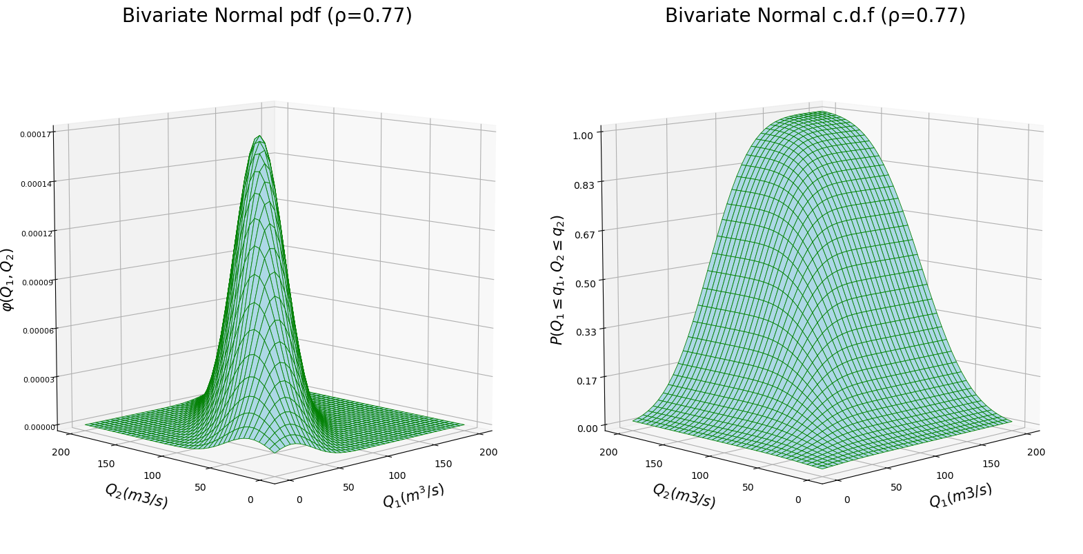
Fig. 4 Bivariate Gaussian distribution: (left) probability density function, and (right) cumulative distribution function.

Conditionalizing a bivariate Gaussian distribution

Multivariate Gaussian distributions are convenient because we can derive results analytically. Here, we are going to conditionalize a bivariate Gaussian distribution to exemplify it.

Given that we are modelling the joint probability distribution of \(X_1\) and \(X_2\) using a bivariate Gaussian distribution and we know \(x_2=a\), what is the expected distribution for \(X_1\)?

An important property of the multivariate Gaussian distribution is that if two sets of variables are jointly Gaussian, then the conditional distribution of one set conditioned on the other is again Gaussian. Thus, the conditional distribution of \(X_1\) given the value of \(X_2\) will be a Gaussian distribution whose mean value (\(\hat{\mu}\)) and standard deviation (\(\hat{\Sigma}\)) we need to estimate. This is, we want to compute \((x_1|x_2=a)\sim N(\hat{\mu}, \hat{\Sigma})\). We can derive expressions for \(\hat{\mu}\) and \(\hat{\Sigma}\) applying the definition of conditional density \(\phi(x_1|x_2=a)=\frac{f_{X_1,X_2}(x_1, a)}{f_{X_2}(a)}\) knowing that \(f_{X_1,X_2}\) is a bivariate Gaussian distribution and \(f_{X_2}\) is a univariate Gaussian distribution, replacing \(x_2\) by \(a\) and doing the (unpleasant) algebra. By doing so, we would reach the following expressions:

\[ \hat{\mu}=\mu_1+\Sigma_{12}\Sigma_{22}^{-1}(a-\mu_2) \]

\[ \hat{\Sigma}=\Sigma_{11}-\Sigma_{12}\Sigma_{22}^{-1}\Sigma_{21} \]

where \(a\) is the known value of \(X_2\) and \(\boldsymbol{\Sigma}=\begin{pmatrix} \Sigma_{11} \ \Sigma_{12} \\ \Sigma_{21} \ \Sigma_{22} \end{pmatrix}\).

Let’s now think of an example of application. Consider the discharge of two rivers,\(Q_{1}\) and \(Q_{2}\), that are located in the same watershed, which will serve as our two random variables. Since the rivers are located in the same watershed, it is relatively safe to assume that their discharges are correlated. We have historical measurements for both discharges and we want to apply a bivariate Gaussian distribution to model their joint distribution. Using the historical dataset, we can compute their mean values, \(\mu_1=94 m^3/s\) and \(\mu_2=78 m^3/s\), their standard deviations, \(\sigma_1= 41 m^3/s\) and \(\sigma_2=35 m^3/s\), and the covariance between them, \(Cov(Q_1, Q_2)=1000 (m^3/s)^2\). We know that \(q_2=100 m^3/s\). What is then the expected distribution for \(Q_1\)? This is, we want to compute \((q_1|q_2=100m^3/s)\sim N(\hat{\mu}, \hat{\Sigma})\).

We can summarize the above information as

\[\begin{split} \boldsymbol{\mu} = \begin{pmatrix} 94 \\ 78\end{pmatrix} \end{split}\]

\[\begin{split} \boldsymbol{\Sigma} = \begin{pmatrix} 41^2 \ 1000 \\ 1000 \ 35^2\end{pmatrix}\end{split}\]

Using the above expressions to our examples, we obtain

\[ \hat{\mu} = 94 + 1000 \times (35^2)^{-1} \times (100-78) \approx 112.0 \]

\[ \hat{\Sigma} = 41^2 - 1000 \times (35^2)^{-1} \times 1000 \approx 864.7 \to \sigma_{x_1|x_2=a}=29.4 \]

The figure below displays the difference between the univariate distribution of \(Q_1\) and the conditional distribution of \(Q_1\) given \(q_2 = 100 m^3/s\).

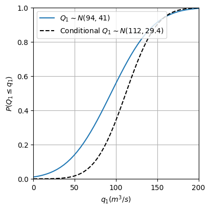
Fig. 5 Distribution of \(Q_1\) and conditional distribution of \(Q_1\) given \(Q_2\). .

From 2D to 3D: multivariate margins

Often in the fields of Civil Engineering and Geosciences, we want to model more than two variables. Sometimes even tens or hundreds of variables. Thus, we need to find flexible models that account for the probabilistic dependence between them the best way possible. One option is to extend the bivariate Gaussian distribution to a multivariate Gaussian distribution with the desired number of random variables. Note that this implies that all the random variables are Gaussian-distributed.

We can extend the analytical equation to conditionalize the bivariate Gaussian distribution to the 3D multivariate Gaussian distribution to compute \((x_1, x_2|x_3=a)\sim N(\hat{\mu}, \hat{\Sigma})\) as

\[\begin{split} \hat{\mu} = \begin{pmatrix} \mu_1 \\ \mu_2 \end{pmatrix} + \begin{pmatrix} \Sigma_{13} \\ \Sigma_{23} \end{pmatrix} \Sigma_{33}^{-1} (a - \mu_3) \end{split}\]

\[\begin{split} \hat{\Sigma} = \begin{pmatrix} \Sigma_{11} \Sigma_{12} \\ \Sigma_{21} \Sigma_{22} \end{pmatrix} - \begin{pmatrix} \Sigma_{13} \\ \Sigma_{23} \end{pmatrix} \Sigma_{33}^{-1} \begin{pmatrix} \Sigma_{13} \ \Sigma_{23}\end{pmatrix} \end{split}\]

Let’s see an example with three dimensions. Imagine that we want to model the dependence between the precipitation, \(P\), and the discharges of the two rivers, \(Q_1\) and \(Q_2\). From a raingauge station, we could obtain the needed statistics of \(P\) to model it using a Gaussian distribution, \(\mu_P=12mm/h\) and \(\sigma_P=27mm/h\), as well as the covariance with \(Q_1\) and \(Q_2\), \(Cov(P, Q_1)=475\) and \(Cov(P, Q_2)=520\). Assuming that we model the joint distribution of \(P\), \(Q_1\) and \(Q_2\) using a multivariate Gaussian distribution, its parameters would be

\[\begin{split} \boldsymbol{\mu} = \begin{pmatrix} 94 \\ 78 \\ 12 \end{pmatrix} \end{split}\]

\[\begin{split} \boldsymbol{\Sigma} = \begin{pmatrix} 41^2 \ 1000 \ 475 \\ 1000 \ 35^2 \ 520\\ 475 \ 520 \ 27^2\end{pmatrix}\end{split}\]

Now we want to make use of the multivariate Gaussian distribution to see what is the distribution of the discharges in the river if today is raining \(p = 22mm/h\). This is, we are going to conditionalize the 3D multivariate Gaussian on one variable, \(P\), to obtain a conditional bivariate Gaussian distribution of \(Q_1\) and \(Q_2\). In mathematical terms, \((q_1, q_2|p=22mm/h)\sim N(\hat{\mu}, \hat{\Sigma})\). We would do it as

\[\begin{split} \hat{\mu} = \begin{pmatrix} 94 \\ 78 \end{pmatrix} + \begin{pmatrix} 475 \\ 520 \end{pmatrix} (27^2)^{-1} (22 - 12) = \begin{pmatrix} 100.5 \\ 85.1 \end{pmatrix} \end{split}\]

\[\begin{split} \hat{\Sigma} = \begin{pmatrix} 41^2 \ 1000 \\ 1000 \ 35^2 \end{pmatrix} - \begin{pmatrix} 475 \\ 520 \end{pmatrix} (27^2)^{-1} \begin{pmatrix} 475 \ 520\end{pmatrix} = \begin{pmatrix} 41^2 \ 1000 \\ 1000 \ 35^2 \end{pmatrix} - \begin{pmatrix} 309.5 \ 338.8 \\ 338.8 \ 370.9 \end{pmatrix} = \begin{pmatrix} 1372.5 \ 661.2 \\ 661.2 \ 854.1 \end{pmatrix} \end{split}\]

We can see that the means of the random variables \(Q_1\) and \(Q_2\) have increased while \(Cov(Q_1, Q_2)\) has been reduced from 1000 to 661.2. The figure below displays the difference between the univariate distributions of \(Q_1\) and \(Q_2\) without and with conditionalizing.

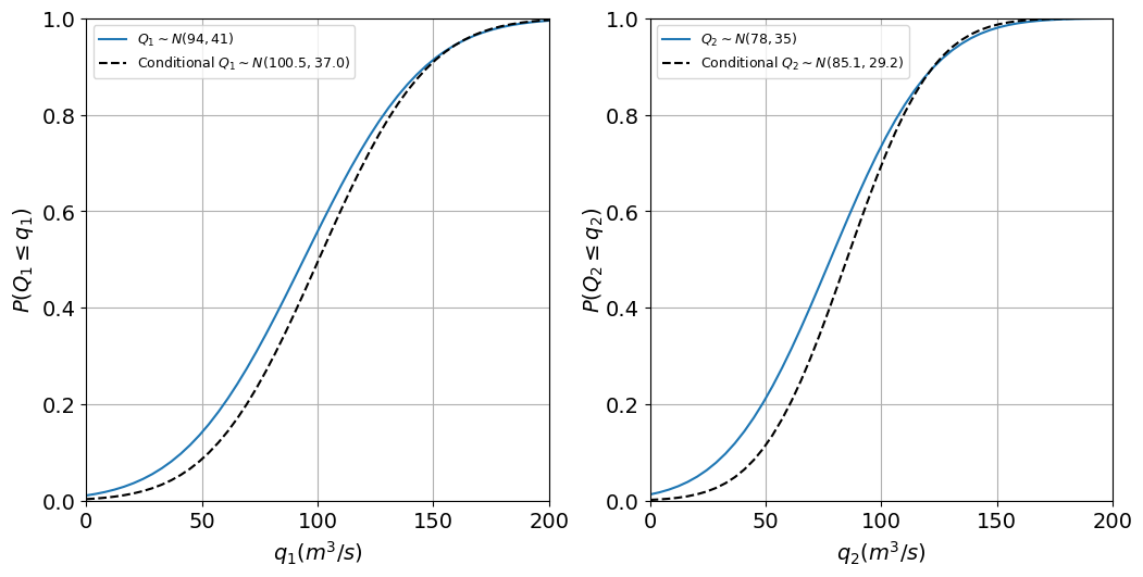
Fig. 6 Unconditional and conditional Gaussian distributions given \(P\): (left) \(Q_1\), and (right) \(Q_2\).

We can also compare the bivariate Gaussian distribution of \(Q_1\) and \(Q_2\) without and with the conditionalization, as shown in the Figure below. You can see how the mode of the distribution (point of maximum density) has moved towards the upper right side of the plot and become slightly narrower when conditionalizing. This is because the three variables are positively correlated and we have conditionalized on a value of precipitation higher than the mean.

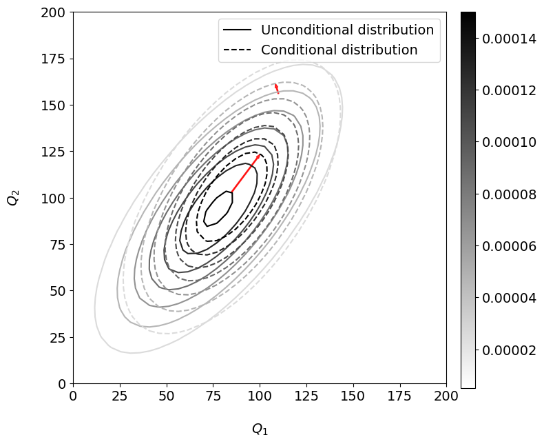
Fig. 7 Unconditional and conditional bivariate Gaussian distributions for \(Q_1\) and \(Q_2\). Same density contours are plotted for both distributions. The small red arrows indicate the shift in the joint probability contours.

Extra material: a video

If you need to refresh the concept of covariance and correlation and want to see a short video on the multivariate Gaussian distribution, you have one here!

Your turn now!

Exercise: Keep your bike chain clean

Considering that you are living in the Netherlands, most probably, you are riding a bike everyday. You can imagine that your bike parts will deteriorate over time and, at some point, they will break. Also, the failure of a part in the mechanism may cause a subsequent failure of a different part connected to it. For example, the failure of the chain might damage the rear cassette and vice versa. In this exercise, we are going to model the number of hours of riding until the failure of parts of the bike.

Let’s now say that the companies that design these parts inform us that the distribution of the number of hours of riding until failure for students from TU Delft is a Gaussian distribution with \(\mu_{T_{chain}} = 1700 hr\) and \(\sigma_{T_{chain}} = 600 hr\) for the number of hours until the chain breaks (\(T_{chain}\)), and \(\mu_{T_{cassette}} = 1300 hr\) with \(\sigma_{T_{cassette}} = 850 hr\) for the number of hours until the cassette breaks (\(T_{casette}\)). Also, we find that \(Cov(T_{chain},T_{cassette}) = 336000\) hours\(^2\).

Compute Pearson’s correlation coefficient between \(T_{chain}\) and \(T_{cassette}\)

\[ \rho_{T_{chain}, T_{cassette}} = \frac{Cov(T_{chain}, T_{cassette})}{\sigma_{T_{chain}} \sigma_{T_{cassette}}} = \frac{336000}{600 \times 850} \approx 0.66 \]

Define the covariance matrix for \(T_{chain}\) and \(T_{cassette}\)

\[\begin{split} \Sigma = \begin{pmatrix} 600^2 \ \ \ 336000 \\ 336000 \ \ \ 850^2 \end{pmatrix} \end{split}\]

The former information depends also on how regularly the students are cleaning the bike, which is not always that frequently. It is obvious that a rusting chain, due to its exposure in the typical Dutch weather, will not be as strong as its brand new version. Let’s say that the mean number of bike cleaning days for a student of TU Delft in a year is \(\mu_{T_{clean}} = 12 \ days\) (that much?) and \(\sigma_{T_{clean}} = 6.3 \ days\). You also know the relationship between the \(T_{clean}\), \(T_{chain}\) and \(T_{cassette}\) defined by \(Cov(T_{clean},T_{chain}) = 2835 \ h \cdot days\) and \(Cov(T_{clean},T_{cassette}) = 3748.5 \ h \cdot days\).

Assuming that \(F(T_{chain}, T_{cassette}, T_{clean})\) follows a multivariate Gaussian distributions, compute the parameters of the conditional bivariate distribution of \(T_{chain}\) and \(T_{cassette}\) for a student that cleans the bike only 7 days per year.

Solution

Initial distribution:

The parameters of the multivariate Gaussian distribution are the mean vector \(\boldsymbol{\mu}\) and the covariance matrix \(\boldsymbol{\Sigma}\) that are given by

\[\begin{split} \boldsymbol{\mu} = \begin{pmatrix} 1700 \\ 1300 \\ 12 \end{pmatrix} \end{split}\]

\[\begin{split} \boldsymbol{\Sigma} = \begin{pmatrix} 600^2 \ 336000 \ 2835 \\ 336000 \ 850^2 \ 3748.5\\ 2835 \ 3748.5 \ 6.3^2\end{pmatrix}\end{split}\]

If we know that \(T_{clean}\) = 7 days, we can conditionalize the multivariate Gaussian distribution as:

\[\begin{split} \hat{\mu} = \begin{pmatrix} 1700 \\ 1300 \end{pmatrix} + \begin{pmatrix} 2835 \\ 3748.5 \end{pmatrix} (6.3^2)^{-1} (7 - 12) = \begin{pmatrix} 1342.6 \\ 827.8 \end{pmatrix} \end{split}\]

\[\begin{split} \hat{\Sigma} = \begin{pmatrix} 600^2 \ 336000 \\ 336000 \ 850^2 \end{pmatrix} - \begin{pmatrix} 2835 \\ 3748.5 \ \end{pmatrix} (6.3^2)^{-1} \begin{pmatrix} 2835 \ 3748.5\end{pmatrix} = \begin{pmatrix} 600^2 \ 336000 \\ 336000 \ 850^2 \end{pmatrix} - \begin{pmatrix} 202500 \ 267750 \\ 267750 \ 354025 \end{pmatrix} = \begin{pmatrix} 157500 \ 68250 \\ 68250 \ 368475 \end{pmatrix} \end{split}\]

Still want more?

Use the multivariate Gaussian distribution implemented in Scipy.stats to plot the density contours of the conditional and unconditional bivariate distributions. How has the distribution changed?

---

[1]

You can check the definition of covariance here.